Difference between revisions of "Magnetostriction"
| Line 5: | Line 5: | ||
To run the model, open '''choke.pro''' with Gmsh. | To run the model, open '''choke.pro''' with Gmsh. | ||
| − | This 2D model | + | This 2D model computes the mechanical deflection of a two columns inductor. It takes into account: |
* The magnetostriction effect in magnetic sheets | * The magnetostriction effect in magnetic sheets | ||
* The Maxwell stress tensor into the whole domain (Airgap and magnetic core) | * The Maxwell stress tensor into the whole domain (Airgap and magnetic core) | ||
| − | Magnetic and mechanical physics are weakly coupled and assume that mechanical deflections | + | Magnetic and mechanical physics are weakly coupled and assume that mechanical deflections do not modify the magnetic field. |
| − | In this way, | + | In this way, the magnetic field is first computed, and the Maxwell stress tensor as well as the magnetostriction strain tensor are deduced from this simulation. |
| − | + | These two tensors are then injected in the mechanical simulation to obtain the deflection. | |
| − | The mecanical model allows | + | The mecanical model also allows to estimate the different resonant frequencies or the inductor. |
| − | + | File details: | |
| − | * choke.geo: the geometry which is parametrized | + | * choke.geo: the geometry, which is parametrized |
| − | * choke.pro: | + | * choke.pro: pro File associated to choke.geo |
| − | * Elasticity_2D.pro: | + | * Elasticity_2D.pro: the mechanical physics |
| − | * magnetostriction.txt: | + | * magnetostriction.txt: the magnetostriction curve |
| − | * jacobian.pro: | + | * jacobian.pro: the integration and Jacobian methods |
| − | * Magsta2D.pro: | + | * Magsta2D.pro: the electromagnetic physics |
== Assumptions== | == Assumptions== | ||
| Line 28: | Line 28: | ||
== Geometry == | == Geometry == | ||
| − | A two columns inductor is | + | A two columns inductor is modelled and the geometry can be modified using parameters: |
| − | * | + | * column height |
| − | * | + | * column width |
| − | * | + | * number of airgap |
* airgap thichness | * airgap thichness | ||
* yoke length | * yoke length | ||
* winding thickness | * winding thickness | ||
| − | |||
| − | |||
== Boundaries == | == Boundaries == | ||
| − | === | + | === Magnetic === |
| − | The magnectic vector potential ''a'' is fixed to 0 | + | The magnectic vector potential ''a'' is fixed to 0 on the external boundaries of the system. |
The current density is imposed into the winding and deduced thanks to the nominal current, the number of turns and the cross section of the winding. | The current density is imposed into the winding and deduced thanks to the nominal current, the number of turns and the cross section of the winding. | ||
=== Mechanical === | === Mechanical === | ||
| − | The inferior yoke is assumed fixed ''u=0'' | + | The inferior yoke is assumed fixed (displacement ''u=0''). |
== Magnetics == | == Magnetics == | ||
| − | A 2D Magnetostatic solver is used for this study. | + | A 2D Magnetostatic solver is used for this study. The model computes the magnectic vector potential ''a''. |
| − | Materials are considered linear and sources of currents are directly imposed. The solver is | + | Materials are considered linear and sources of currents are directly imposed. The solver is coded in the file '''MagSta_2D.pro''' |
<math> | <math> | ||
| Line 61: | Line 59: | ||
</math> | </math> | ||
| − | Different post-proccessing are | + | Different post-proccessing are predefined: |
| − | * The | + | * The flux density B |
| − | * The | + | * The magnetic field H |
| − | * The | + | * The energy per length unit (J/m) |
| Line 89: | Line 87: | ||
== Magnetostriction strain tensor == | == Magnetostriction strain tensor == | ||
| − | The magnetostriction tensor is obtained using the flux density map and with the magnetostriction curve of the material witch | + | The magnetostriction tensor is obtained using the flux density map and with the magnetostriction curve of the material witch links the strain with the flux density. This kind of curve is presented on the following figure: |
[[File:magnetostriction_curve.png|center|800px]] | [[File:magnetostriction_curve.png|center|800px]] | ||
| − | The curve | + | The curve permits to determine the strain tensor in the referential (Bt,Bn) presented below: |
[[File:referentiel.png|center]] | [[File:referentiel.png|center]] | ||
| Line 109: | Line 107: | ||
</math> | </math> | ||
| − | In order to be injected into the mechanical model, the strain tensor needs to be converted into the (x,y) basis. This is done by computing the change of basis matrix P. In this way the strain tensor in the basis (x,y) is | + | In order to be injected into the mechanical model, the strain tensor needs to be converted into the (x,y) basis. This is done by computing the change of basis matrix P. In this way the strain tensor in the basis (x,y) is determined: |
<math> | <math> | ||
| Line 163: | Line 161: | ||
== Mechanical == | == Mechanical == | ||
| − | A 2D mechanical solver is added to the model. | + | |
| + | A 2D mechanical solver is added to the model. This harmonic solver permits to compute the deflection of the inductor due to the magnetostriction and the Maxwell stress tensor. It also permits to obtain the eigen modes of the magnetic core. No damping is currently added so that resonnance are not ... | ||
| Line 170: | Line 169: | ||
4 resolution methods are provided: | 4 resolution methods are provided: | ||
* A magnetostatic study | * A magnetostatic study | ||
| − | * A magneto-mechanical study with | + | * A magneto-mechanical study with allows to estimate the complete deflection of the magnetic core due to magnetic effects |
| − | * A magneto-mechanical study on a specific point. It | + | * A magneto-mechanical study on a specific point. It computes the deflection of a specific point. It is the same procedure as the previous point but allow easily to compute the FRF on a specific point. It shows that magnetostriction and/or Maxwell dtress tensor can stimulate a resonnance |
| − | * A mechanical study to obtain the eigen mode | + | * A mechanical study to obtain the eigen mode of the inductor. |
| − | |||
| − | |||
| − | |||
Revision as of 10:19, 23 April 2015
|
2D model of inductor with magnetostriction.
|
|
|---|
|
Download model archive (magnetostriction.zip) |
Contents
Introduction
To run the model, open choke.pro with Gmsh.
This 2D model computes the mechanical deflection of a two columns inductor. It takes into account:
- The magnetostriction effect in magnetic sheets
- The Maxwell stress tensor into the whole domain (Airgap and magnetic core)
Magnetic and mechanical physics are weakly coupled and assume that mechanical deflections do not modify the magnetic field. In this way, the magnetic field is first computed, and the Maxwell stress tensor as well as the magnetostriction strain tensor are deduced from this simulation. These two tensors are then injected in the mechanical simulation to obtain the deflection.
The mecanical model also allows to estimate the different resonant frequencies or the inductor.
File details:
- choke.geo: the geometry, which is parametrized
- choke.pro: pro File associated to choke.geo
- Elasticity_2D.pro: the mechanical physics
- magnetostriction.txt: the magnetostriction curve
- jacobian.pro: the integration and Jacobian methods
- Magsta2D.pro: the electromagnetic physics
Assumptions
Geometry
A two columns inductor is modelled and the geometry can be modified using parameters:
- column height
- column width
- number of airgap
- airgap thichness
- yoke length
- winding thickness
Boundaries
Magnetic
The magnectic vector potential a is fixed to 0 on the external boundaries of the system. The current density is imposed into the winding and deduced thanks to the nominal current, the number of turns and the cross section of the winding.
Mechanical
The inferior yoke is assumed fixed (displacement u=0).
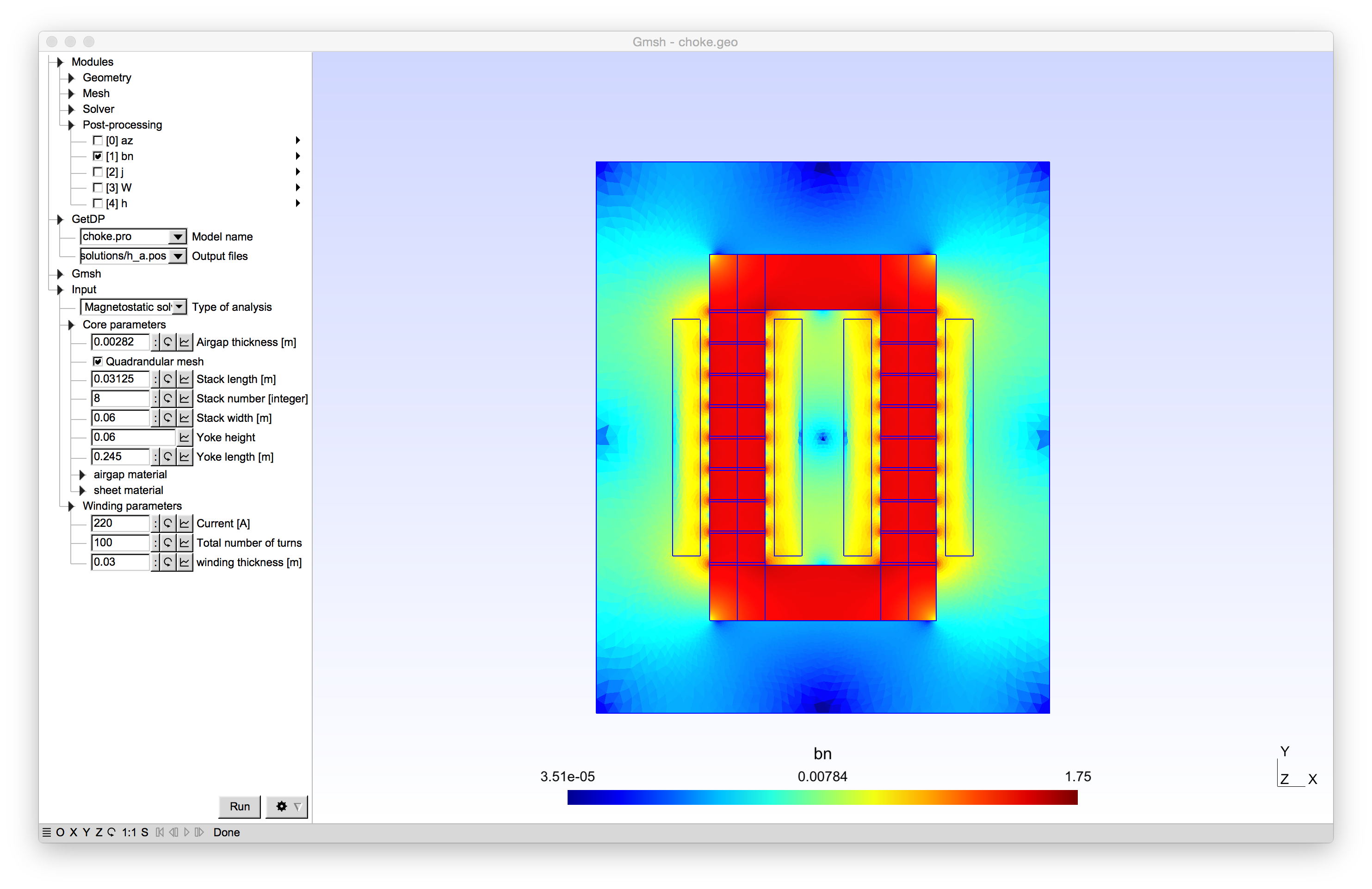
Magnetics
A 2D Magnetostatic solver is used for this study. The model computes the magnectic vector potential a. Materials are considered linear and sources of currents are directly imposed. The solver is coded in the file MagSta_2D.pro
\( \begin{eqnarray} \nabla^2 \mathbf{A} + \mu_0 \mu_r \mathbf{j_z} = \mathbf{0} \label{eq:vector_potential} \end{eqnarray} \)
Different post-proccessing are predefined:
- The flux density B
- The magnetic field H
- The energy per length unit (J/m)
Maxwell Stress Tensor
The Maxwell Stress Tensor is deduced directly from the magnetic field and is injected into the mechanical solver.
\(\begin{eqnarray} \sigma_{mst}= \frac{1}{\mu_0\mu_r}\begin{bmatrix} B_x^2 -\frac{1}{2}B^2 & B_xB_y\\ B_xB_y & B_y^2 -\frac{1}{2}B^2 \end{bmatrix} \label{eq:stress} \end{eqnarray}\)
The following code in used :
 sig_maxwell[]=Vector[ CompX[$1]*CompX[$1]-Norm[$1]*Norm[$1]/2,
		       CompY[$1]*CompY[$1]-Norm[$1]*Norm[$1]/2,
		       CompX[$1]*CompY[$1]];
Magnetostriction strain tensor
The magnetostriction tensor is obtained using the flux density map and with the magnetostriction curve of the material witch links the strain with the flux density. This kind of curve is presented on the following figure:

The curve permits to determine the strain tensor in the referential (Bt,Bn) presented below:
The strain tensor is decomposed into two phenomenas: the normal and tangential magnetostriction, called respectively \(\lambda_N\) and \(\lambda_T\). \(\lambda_T\) could be obtained using experimental data, or by asuming that magnetostriction doesn't modify the volume, a simple relation is obtained\[\lambda_N=-\lambda_N/2\]
\( \begin{eqnarray} \epsilon_{(B_t,B_n)}=\begin{bmatrix} \lambda_T & 0 \\ 0 & \lambda_N \end{bmatrix} \label{eq:strain_tensor1} \end{eqnarray} \)
In order to be injected into the mechanical model, the strain tensor needs to be converted into the (x,y) basis. This is done by computing the change of basis matrix P. In this way the strain tensor in the basis (x,y) is determined\[ \begin{eqnarray} P=\begin{bmatrix} \frac{B_x}{B} & -\frac{B_y}{B} \\ \frac{B_y}{B} & \frac{B_x}{B} \\ \end{bmatrix} \label{eq:P} \end{eqnarray} \]
\( \begin{eqnarray} \epsilon_{(x,y)}=P \epsilon_{(B_t,B_n)}\ P^t \label{eq:PPT} \end{eqnarray} \)
\( \begin{eqnarray} \epsilon_{(x,y)}=\begin{bmatrix} \frac{1}{B^2}(\lambda_T B_x^2+\lambda_N B_y^2) & \frac{B_xB_y}{B^2}(\lambda_T-\lambda_N) \\ \frac{B_xB_y}{B^2}(\lambda_T-\lambda_N) & \frac{1}{B^2}(\lambda_T B_y^2+\lambda_N B_x^2) \\ \end{bmatrix} \label{eq:strain_xyz} \end{eqnarray} \)
The following code in used :
lamb[]=Vector[lambdap[Norm[$1]],lambdaper[Norm[$1]],0];

sig_vect[]=C_m[]*lamb[$1];

sig_mat[]=Tensor[CompX[sig_vect[$1]], CompZ[sig_vect[$1]]  ,   0,
	         CompZ[sig_vect[$1]], CompY[sig_vect[$1]]  ,   0,
		            0	    ,          0	   ,   0 ];

// Change of basis

P[]=Tensor[ CompX[$1]/Norm[$1]  ,   -CompY[$1]/Norm[$1] , 0,
            CompY[$1]/Norm[$1]  ,    CompX[$1]/Norm[$1] , 0,
                       0        ,             0         , 1 ];
PP[]=Transpose[P[$1]];
sig_PPP[]=P[$1]*sig_mat[$1]*PP[$1];
sig_magnetostriction[]=Vector[CompXX[sig_PPP[$1]],CompYY[sig_PPP[$1]],CompXY[sig_PPP[$1]]];
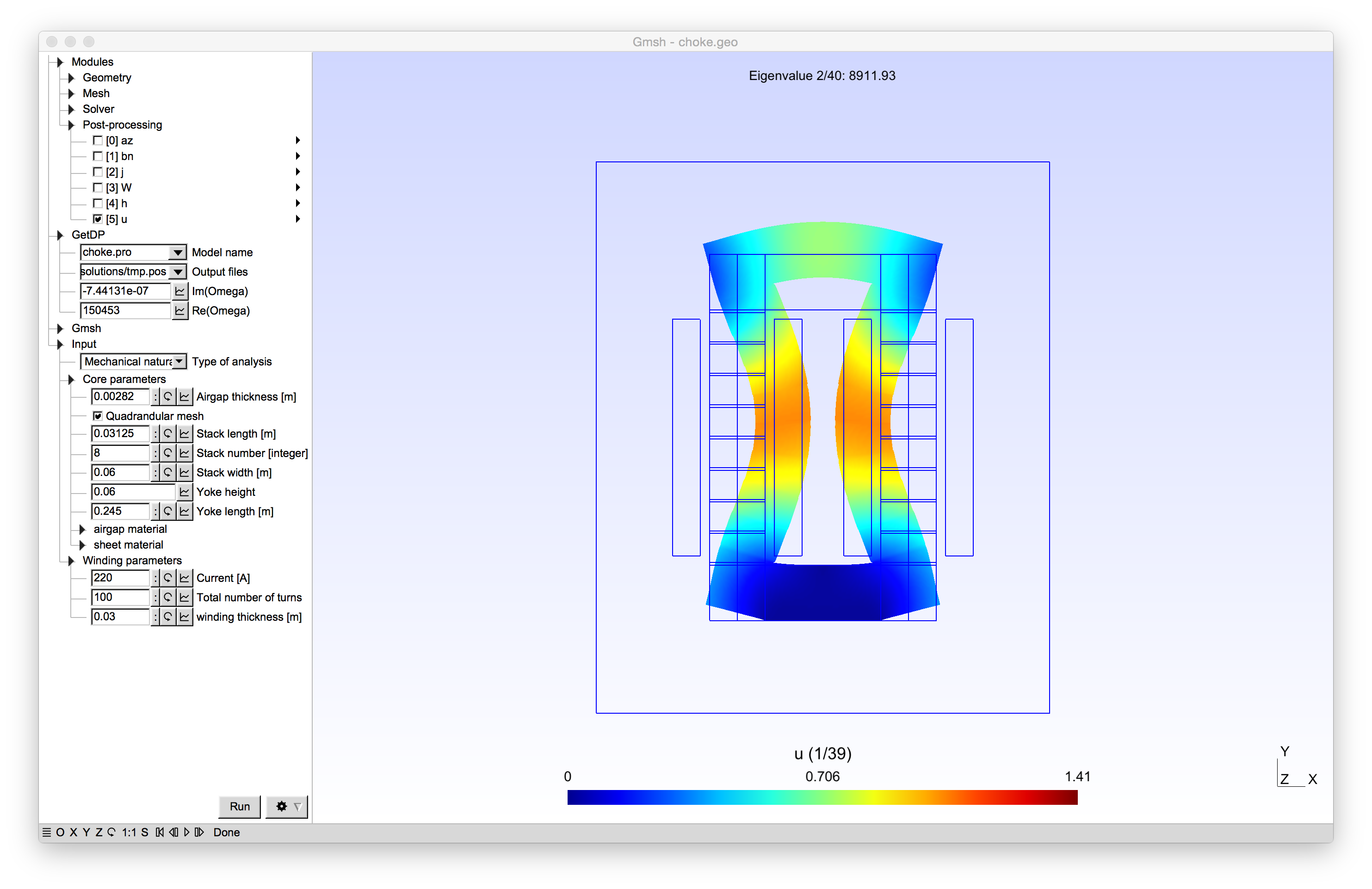
Mechanical
A 2D mechanical solver is added to the model. This harmonic solver permits to compute the deflection of the inductor due to the magnetostriction and the Maxwell stress tensor. It also permits to obtain the eigen modes of the magnetic core. No damping is currently added so that resonnance are not ...
Resolution
4 resolution methods are provided:
- A magnetostatic study
- A magneto-mechanical study with allows to estimate the complete deflection of the magnetic core due to magnetic effects
- A magneto-mechanical study on a specific point. It computes the deflection of a specific point. It is the same procedure as the previous point but allow easily to compute the FRF on a specific point. It shows that magnetostriction and/or Maxwell dtress tensor can stimulate a resonnance
- A mechanical study to obtain the eigen mode of the inductor.
Results
References
|
Models developed by Mathieu Rossi, Jean Le Besnerais and Christophe Geuzaine. Copyright (c) 2015 EOMYS
|