Difference between revisions of "Waveguides"
(Created page with "{{metamodel|waveguides}} {{mytexdefs}} == Introduction == This academic example introduces the numerical solution of eigenvalue problems. The Helmholtz equation (scalar and...") |
|||
| Line 4: | Line 4: | ||
== Introduction == | == Introduction == | ||
| − | |||
| − | |||
| − | |||
| − | |||
| − | |||
| − | |||
$\rightarrow$ To run the example, open '''main.pro''' with Gmsh. | $\rightarrow$ To run the example, open '''main.pro''' with Gmsh. | ||
| Line 15: | Line 9: | ||
== Description of the problem == | == Description of the problem == | ||
| − | ==== | + | ==== Classical waveguides ==== |
| + | |||
| + | :{| class="toccolours mw-collapsible mw-collapsed" width="80%" style="text-align:left" | ||
| + | !General waveguide | ||
| + | |- | ||
| + | | Let us consider a hollow cylindrical waveguide of arbitrary cross-sectional shape that has a principal axis in the $z$-direction. | ||
| + | The elementary solution of this problem reads | ||
| + | \begin{align} | ||
| + | {\bf E}(x,y,z,t) &= {\bf E}(x,y) \: e^{i(\pm kz-\omega t)} \\ | ||
| + | {\bf H}(x,y,z,t) &= {\bf H}(x,y) \: e^{i(\pm kz-\omega t)} | ||
| + | \end{align} | ||
| + | where the new unknowns are governed by | ||
| + | \begin{align} | ||
| + | \left[\nabla_t^2 + (\mu\varepsilon\omega^2 - k^2)\right] \left\{\begin{array}{x}{\bf E}\\{\bf H}\end{array}\right\} = 0 | ||
| + | \end{align} | ||
| + | where $\nabla_t$ is the transverse part of the Nabla operator. | ||
| + | |||
| + | ''' Parallel and transverse fields ''' | ||
| + | |||
| + | It is useful to separate the fields into components parallel to and transverse to the $z$-direction: | ||
| + | \begin{align} | ||
| + | {\bf E} &= {\bf E}_z + {\bf E}_t && \text{with } {\bf E}_z = {E}_z \hat{\bf z} \\ | ||
| + | {\bf H} &={\bf H}_z + {\bf H}_t && \text{with } {\bf H}_z = {H}_z \hat{\bf z} | ||
| + | \end{align} | ||
| + | |||
| + | Some well-known cases: | ||
| + | * Transverse electromagnetic (TEM) waves: if ${E}_z=0$ and ${H}_z=0$ everywhere | ||
| + | * Transverse magnetic (TM) waves: if ${H}_z=0$ everywhere | ||
| + | * Transverse electric (TE) waves: if ${E}_z=0$ everywhere | ||
| + | |||
| + | If both parallel fields are vanishing (TEM case), the transverse fields are the solution of an electrostatic problem in two dimensions. | ||
| + | |||
| + | If at least one parallel field is non-vanishing, the transverse fields are | ||
| + | \begin{align} | ||
| + | {\bf E}_t &= \frac{i}{\mu\varepsilon\omega^2-k^2} \left[\pm\:k\:\nabla_t{E}_z - \mu\omega\:\hat{\bf z}\times\nabla_t{H}_z\right] \\ | ||
| + | {\bf H}_t &= \frac{i}{\mu\varepsilon\omega^2-k^2} \left[\pm\:k\:\nabla_t{H}_z + \varepsilon\omega\:\hat{\bf z}\times\nabla_t{E}_z\right] | ||
| + | \end{align} | ||
| + | |||
| + | In TEM, TM and TE cases, the transverse fields are related by | ||
| + | \begin{equation} | ||
| + | {\bf H}_t = \pm\frac{1}{Z} \hat{\bf z}\times{\bf E}_t | ||
| + | \end{equation} | ||
| + | where the wave impedance $Z$ is given by | ||
| + | \begin{equation} | ||
| + | Z= | ||
| + | \left\{\begin{array}{ll} | ||
| + | \sqrt{\frac{\mu}{\varepsilon}} &\quad \text{(TEM case)} \\ | ||
| + | \frac{k}{k_0} \sqrt{\frac{\mu}{\varepsilon}} &\quad \text{(TM case)} \\ | ||
| + | \frac{k_0}{k} \sqrt{\frac{\mu}{\varepsilon}} &\quad \text{(TE case)} | ||
| + | \end{array}\right. | ||
| + | \end{equation} | ||
| + | with $k_0=\omega\sqrt{\mu\varepsilon}$. | ||
| + | |||
| + | ''' Eigenvalue problem ''' | ||
| + | |||
| + | For a waveguide with perfectly conducting borders, the non-vanishing parallel field of TM and TE cases | ||
| + | is governed by, respectively, | ||
| + | \begin{align} | ||
| + | \left[\nabla_t^2 + \gamma^2\right] {E}_z &= 0 \\ | ||
| + | \left[\nabla_t^2 + \gamma^2\right] {H}_z &= 0 | ||
| + | \end{align} | ||
| + | with $\gamma^2 = \mu\varepsilon\omega^2 - k^2$, | ||
| + | and is subject to the homogeneous boundary condition ${E}_z=0$ (TM case) or ${\bf n}\cdot\nabla{H}_z = 0$ (TE case). | ||
| + | |||
| + | These equations define eigenvalue problems. | ||
| + | There is a spectrum of eigenvalues $\gamma^2_\ell$ and corresponding solutions $\left.E_z\right|_\ell$ or $\left.H_z\right|_\ell$, $\ell=1,2,...$, | ||
| + | which form an orthogonal set. For a given frequency $\omega$, the wave number $k$ is determined for each $\ell$: | ||
| + | \begin{equation} | ||
| + | k_\ell | ||
| + | = \sqrt{\mu\varepsilon\omega^2-\gamma^2_\ell} | ||
| + | = \sqrt{\mu\varepsilon} \sqrt{\omega^2-\omega^2_\ell} | ||
| + | \end{equation} | ||
| + | where $\omega_\ell$ is the cutoff frequency, defined by | ||
| + | \begin{equation} | ||
| + | \omega_\ell=\frac{\gamma_\ell}{\sqrt{\mu\varepsilon}} | ||
| + | \end{equation} | ||
| + | This frequency defines the nature of waves: | ||
| + | * If $\omega>\omega_\ell$, $k_\ell$ is real and the waves are travelling modes. | ||
| + | * If $\omega<\omega_\ell$, $k_\ell$ is imaginary and the waves are evanescent modes. | ||
| + | |} | ||
| + | |||
| + | :{| class="toccolours mw-collapsible mw-collapsed" width="80%" style="text-align:left" | ||
| + | !Rectangular waveguide | ||
| + | |- | ||
| + | | Let us consider a rectangular waveguide $(x,y)\in[0,a]\times[0,b]$ | ||
| + | that has a principal axis in the $z-$direction. | ||
| + | * For TM modes, the solutions for $E_z$ are | ||
| + | \begin{align} | ||
| + | \left.E_z\right|_{mn} &= E_0 \sin\left(\frac{m\pi x}{a}\right) \sin\left(\frac{n\pi y}{b}\right) e^{ikz-i\omega t} && \text{with } m,n=0,1,2,... | ||
| + | \end{align} | ||
| + | * For TE modes, the solutions for $H_z$ are | ||
| + | \begin{align} | ||
| + | \left.H_z\right|_{mn} &= H_0 \cos\left(\frac{m\pi x}{a}\right) \cos\left(\frac{n\pi y}{b}\right) e^{ikz-i\omega t} && \text{with } m,n=0,1,2,... | ||
| + | \end{align} | ||
| + | In both cases, the eigenvalues and the cutoff frequencies are, respectively, | ||
| + | \begin{align} | ||
| + | \gamma_{mn}^2 &= \pi^2\left(\frac{m^2}{a^2}+\frac{n^2}{b^2}\right) && \text{with } m,n=0,1,2,... \\ | ||
| + | \omega_{mn}^2 &= \frac{\pi}{\sqrt{\mu\varepsilon}}\sqrt{\frac{m^2}{a^2}+\frac{n^2}{b^2}} && \text{with } m,n=0,1,2,... | ||
| + | \end{align} | ||
| + | The complete solution for the TM<sub>10</sub> and TE<sub>10</sub> modes are, respectively, | ||
| + | \begin{align} | ||
| + | \begin{cases} | ||
| + | \displaystyle E_z = E_0 \sin\left(\frac{\pi x}{a}\right) e^{ikz-i\omega t} \\ | ||
| + | \displaystyle E_x = i\frac{ka}{\pi} E_0 \cos\left(\frac{\pi x}{a}\right) e^{ikz-i\omega t} \\ | ||
| + | \displaystyle H_y = i\frac{\varepsilon\omega a}{\pi} E_0 \cos\left(\frac{\pi x}{a}\right) e^{ikz-i\omega t} | ||
| + | \end{cases} | ||
| + | \quad\quad\text{and}\quad\quad | ||
| + | \begin{cases} | ||
| + | \displaystyle H_z = H_0 \cos\left(\frac{\pi x}{a}\right) e^{ikz-i\omega t} \\ | ||
| + | \displaystyle H_x = -i\frac{ka}{\pi} H_0 \sin\left(\frac{\pi x}{a}\right) e^{ikz-i\omega t} \\ | ||
| + | \displaystyle E_y =i\frac{\mu\omega a}{\pi} H_0 \sin\left(\frac{\pi x}{a}\right) e^{ikz-i\omega t} | ||
| + | \end{cases} | ||
| + | \end{align} | ||
| + | |} | ||
| + | |||
| + | ==== Discontinuities and networks ==== | ||
| + | |||
| + | |||
| + | :{| class="toccolours mw-collapsible mw-collapsed" width="80%" style="text-align:left" | ||
| + | !Discontinuity in a parallel-plate waveguide | ||
| + | |- | ||
| + | | See <ref name=Jin2002 />, section 4.6.1. | ||
| + | |||
| + | * Solution for the TE mode | ||
| + | \begin{align} | ||
| + | H_z &= H_0 e^{-jk_0 x} + R H_0 e^{jk_0 x} && \text{at } x=x_1 \\ | ||
| + | H_z &= T H_0 e^{-jk_0 x} && \text{at } x=x_2 | ||
| + | \end{align} | ||
| + | |||
| + | * Boundary conditions | ||
| + | \begin{align} | ||
| + | \partial_x H_z &= jk_0 H_z - 2jk_0H_0 e^{-jk_0 x} && \text{at } x=x_1 \\ | ||
| + | \partial_x H_z &= -jk_0 H_z && \text{at } x=x_2 | ||
| + | \end{align} | ||
| + | |||
| + | * Reflection and transmission coefficients | ||
| + | \begin{align} | ||
| + | R &= \left.\frac{H_z - H_0 e^{-jk_0x}}{H_0 e^{ jk_0 x}}\right|_{x=x_1} \\ | ||
| + | T &= \left.\frac{H_z}{H_0 e^{-jk_0 x}}\right|_{x=x_2} | ||
| + | \end{align} | ||
| + | : with $|R|^2+|T|^2=1$. | ||
| + | |} | ||
| + | |||
| + | :{| class="toccolours mw-collapsible mw-collapsed" width="80%" style="text-align:left" | ||
| + | !Waveguide with discontinuities | ||
| + | |- | ||
| + | | See <ref name=Jin2002 />, section 8.5. | ||
| + | |||
| + | * Solution for the TE$_{mn}$ mode | ||
| + | \begin{align} | ||
| + | {\bf E}(x,y,z) &= E_0 {\bf e}_{mn}(x,y) e^{-jk_{z_{mn}} z} + R E_0 {\bf e}_{mn}(x,y) e^{jk_{z_{mn}} z} && \text{at } z=z_1 \\ | ||
| + | {\bf E}(x,y,z) &= T E_0 {\bf e}_{mn}(x,y) e^{-jk_{z_{mn}} z} && \text{at } z=z_2 | ||
| + | \end{align} | ||
| + | |||
| + | * Reflection and transmission coefficients | ||
| + | \begin{align} | ||
| + | R &= \left.\frac{{\bf E}(x,y,z) - E_0 {\bf e}_{mn}(x,y) e^{-jk_{z_{10}}z}}{E_0 {\bf e}_{mn}(x,y) e^{jk_{z_{10}}z}}\right|_{z=z_1} \\ | ||
| + | T &= \left.\frac{{\bf E}(x,y,z)}{E_0 {\bf e}_{mn}(x,y) e^{-jk_{z_{10}}z}}\right|_{z=z_2} | ||
| + | \end{align} | ||
| + | : with $|R|^2+|T|^2=1$. | ||
| + | |||
| + | * Reflection and transmission coefficients (improved - the dominant mode $mn$ - using the orthogonality properties of modes) | ||
| + | \begin{align} | ||
| + | R &= \frac{e^{-jk_{z_{mn}}z_1}}{E_0} \frac{\int_{S_1}{\bf E}(x,y,z)\cdot{\bf e}_{mn}(x,y) \: dS}{\int_{S_1}{\bf e}_{mn}(x,y)\cdot{\bf e}_{mn}(x,y) \: dS} - e^{-2jk_{z_{mn}}z_1}\\ | ||
| + | T &= \frac{e^{jk_{z_{mn}}z_2}}{E_0} \frac{\int_{S_2}{\bf E}(x,y,z)\cdot{\bf e}_{mn}(x,y) \: dS}{\int_{S_2}{\bf e}_{mn}(x,y)\cdot{\bf e}_{mn}(x,y) \: dS} | ||
| + | \end{align} | ||
| + | : with $|R|^2+|T|^2=1$. | ||
| + | |} | ||
| + | |||
| + | ==== Numerical resolution ==== | ||
| + | |||
| − | |||
== Some results == | == Some results == | ||
| Line 27: | Line 190: | ||
<references> | <references> | ||
| − | |||
<ref name=Jin2002> J. Jin, ''The Finite Element Method in Electromagnetics''. Second edition. John Wiley & Sons, 2002</ref> | <ref name=Jin2002> J. Jin, ''The Finite Element Method in Electromagnetics''. Second edition. John Wiley & Sons, 2002</ref> | ||
| Line 33: | Line 195: | ||
| − | {{metamodelfooter| | + | {{metamodelfooter|waveguides}} |
Revision as of 11:43, 15 March 2014
|
2D and 3D models of metallic waveguides
|
|
|---|
|
Download model archive (waveguides.zip) |
\(\renewcommand{\vec}[1]{\mathbf{#1}} \newcommand{\Grad}[1]{\mathbf{\text{grad}}\,{#1}} \newcommand{\Curl}[1]{\mathbf{\text{curl}}\,{#1}} \newcommand{\Div}[1]{\text{div}\,{#1}} \newcommand{\Real}[1]{\text{Re}({#1})} \newcommand{\Imag}[1]{\text{Im}({#1})} \newcommand{\pvec}[2]{{#1}\times{#2}} \newcommand{\psca}[2]{{#1}\cdot{#2}} \newcommand{\E}[1]{\,10^{#1}} \newcommand{\Ethree}{{\mathbb{E}^3}} \newcommand{\Etwo}{{\mathbb{E}^2}} \newcommand{\Units}[1]{[\mathrm{#1}]} \)
Contents
Introduction
$\rightarrow$ To run the example, open main.pro with Gmsh.
Description of the problem
Classical waveguides
General waveguide Let us consider a hollow cylindrical waveguide of arbitrary cross-sectional shape that has a principal axis in the $z$-direction. The elementary solution of this problem reads \begin{align} {\bf E}(x,y,z,t) &= {\bf E}(x,y) \: e^{i(\pm kz-\omega t)} \\ {\bf H}(x,y,z,t) &= {\bf H}(x,y) \: e^{i(\pm kz-\omega t)} \end{align} where the new unknowns are governed by \begin{align} \left[\nabla_t^2 + (\mu\varepsilon\omega^2 - k^2)\right] \left\{\begin{array}{x}{\bf E}\\{\bf H}\end{array}\right\} = 0 \end{align} where $\nabla_t$ is the transverse part of the Nabla operator.
Parallel and transverse fields
It is useful to separate the fields into components parallel to and transverse to the $z$-direction: \begin{align} {\bf E} &= {\bf E}_z + {\bf E}_t && \text{with } {\bf E}_z = {E}_z \hat{\bf z} \\ {\bf H} &={\bf H}_z + {\bf H}_t && \text{with } {\bf H}_z = {H}_z \hat{\bf z} \end{align}
Some well-known cases:
- Transverse electromagnetic (TEM) waves: if ${E}_z=0$ and ${H}_z=0$ everywhere
- Transverse magnetic (TM) waves: if ${H}_z=0$ everywhere
- Transverse electric (TE) waves: if ${E}_z=0$ everywhere
If both parallel fields are vanishing (TEM case), the transverse fields are the solution of an electrostatic problem in two dimensions.
If at least one parallel field is non-vanishing, the transverse fields are \begin{align} {\bf E}_t &= \frac{i}{\mu\varepsilon\omega^2-k^2} \left[\pm\:k\:\nabla_t{E}_z - \mu\omega\:\hat{\bf z}\times\nabla_t{H}_z\right] \\ {\bf H}_t &= \frac{i}{\mu\varepsilon\omega^2-k^2} \left[\pm\:k\:\nabla_t{H}_z + \varepsilon\omega\:\hat{\bf z}\times\nabla_t{E}_z\right] \end{align}
In TEM, TM and TE cases, the transverse fields are related by \begin{equation} {\bf H}_t = \pm\frac{1}{Z} \hat{\bf z}\times{\bf E}_t \end{equation} where the wave impedance $Z$ is given by \begin{equation} Z= \left\{\begin{array}{ll} \sqrt{\frac{\mu}{\varepsilon}} &\quad \text{(TEM case)} \\ \frac{k}{k_0} \sqrt{\frac{\mu}{\varepsilon}} &\quad \text{(TM case)} \\ \frac{k_0}{k} \sqrt{\frac{\mu}{\varepsilon}} &\quad \text{(TE case)} \end{array}\right. \end{equation} with $k_0=\omega\sqrt{\mu\varepsilon}$.
Eigenvalue problem
For a waveguide with perfectly conducting borders, the non-vanishing parallel field of TM and TE cases is governed by, respectively, \begin{align} \left[\nabla_t^2 + \gamma^2\right] {E}_z &= 0 \\ \left[\nabla_t^2 + \gamma^2\right] {H}_z &= 0 \end{align} with $\gamma^2 = \mu\varepsilon\omega^2 - k^2$, and is subject to the homogeneous boundary condition ${E}_z=0$ (TM case) or ${\bf n}\cdot\nabla{H}_z = 0$ (TE case).
These equations define eigenvalue problems. There is a spectrum of eigenvalues $\gamma^2_\ell$ and corresponding solutions $\left.E_z\right|_\ell$ or $\left.H_z\right|_\ell$, $\ell=1,2,...$, which form an orthogonal set. For a given frequency $\omega$, the wave number $k$ is determined for each $\ell$: \begin{equation} k_\ell = \sqrt{\mu\varepsilon\omega^2-\gamma^2_\ell} = \sqrt{\mu\varepsilon} \sqrt{\omega^2-\omega^2_\ell} \end{equation} where $\omega_\ell$ is the cutoff frequency, defined by \begin{equation} \omega_\ell=\frac{\gamma_\ell}{\sqrt{\mu\varepsilon}} \end{equation} This frequency defines the nature of waves:
- If $\omega>\omega_\ell$, $k_\ell$ is real and the waves are travelling modes.
- If $\omega<\omega_\ell$, $k_\ell$ is imaginary and the waves are evanescent modes.
Rectangular waveguide Let us consider a rectangular waveguide $(x,y)\in[0,a]\times[0,b]$ that has a principal axis in the $z-$direction.
- For TM modes, the solutions for $E_z$ are
\begin{align} \left.E_z\right|_{mn} &= E_0 \sin\left(\frac{m\pi x}{a}\right) \sin\left(\frac{n\pi y}{b}\right) e^{ikz-i\omega t} && \text{with } m,n=0,1,2,... \end{align}
- For TE modes, the solutions for $H_z$ are
\begin{align} \left.H_z\right|_{mn} &= H_0 \cos\left(\frac{m\pi x}{a}\right) \cos\left(\frac{n\pi y}{b}\right) e^{ikz-i\omega t} && \text{with } m,n=0,1,2,... \end{align} In both cases, the eigenvalues and the cutoff frequencies are, respectively, \begin{align} \gamma_{mn}^2 &= \pi^2\left(\frac{m^2}{a^2}+\frac{n^2}{b^2}\right) && \text{with } m,n=0,1,2,... \\ \omega_{mn}^2 &= \frac{\pi}{\sqrt{\mu\varepsilon}}\sqrt{\frac{m^2}{a^2}+\frac{n^2}{b^2}} && \text{with } m,n=0,1,2,... \end{align} The complete solution for the TM10 and TE10 modes are, respectively, \begin{align} \begin{cases} \displaystyle E_z = E_0 \sin\left(\frac{\pi x}{a}\right) e^{ikz-i\omega t} \\ \displaystyle E_x = i\frac{ka}{\pi} E_0 \cos\left(\frac{\pi x}{a}\right) e^{ikz-i\omega t} \\ \displaystyle H_y = i\frac{\varepsilon\omega a}{\pi} E_0 \cos\left(\frac{\pi x}{a}\right) e^{ikz-i\omega t} \end{cases}
 \quad\quad\text{and}\quad\quad
  \begin{cases}
    \displaystyle H_z = H_0 \cos\left(\frac{\pi x}{a}\right) e^{ikz-i\omega t} \\
    \displaystyle H_x = -i\frac{ka}{\pi} H_0 \sin\left(\frac{\pi x}{a}\right) e^{ikz-i\omega t} \\
    \displaystyle E_y =i\frac{\mu\omega a}{\pi} H_0 \sin\left(\frac{\pi x}{a}\right) e^{ikz-i\omega t}
  \end{cases}
\end{align}
Discontinuities and networks
Discontinuity in a parallel-plate waveguide See [1], section 4.6.1. - Solution for the TE mode
\begin{align} H_z &= H_0 e^{-jk_0 x} + R H_0 e^{jk_0 x} && \text{at } x=x_1 \\ H_z &= T H_0 e^{-jk_0 x} && \text{at } x=x_2 \end{align}
- Boundary conditions
\begin{align} \partial_x H_z &= jk_0 H_z - 2jk_0H_0 e^{-jk_0 x} && \text{at } x=x_1 \\ \partial_x H_z &= -jk_0 H_z && \text{at } x=x_2 \end{align}
- Reflection and transmission coefficients
\begin{align} R &= \left.\frac{H_z - H_0 e^{-jk_0x}}{H_0 e^{ jk_0 x}}\right|_{x=x_1} \\ T &= \left.\frac{H_z}{H_0 e^{-jk_0 x}}\right|_{x=x_2} \end{align}
- with $|R|^2+|T|^2=1$.
Waveguide with discontinuities See [1], section 8.5. - Solution for the TE$_{mn}$ mode
\begin{align} {\bf E}(x,y,z) &= E_0 {\bf e}_{mn}(x,y) e^{-jk_{z_{mn}} z} + R E_0 {\bf e}_{mn}(x,y) e^{jk_{z_{mn}} z} && \text{at } z=z_1 \\ {\bf E}(x,y,z) &= T E_0 {\bf e}_{mn}(x,y) e^{-jk_{z_{mn}} z} && \text{at } z=z_2 \end{align}
- Reflection and transmission coefficients
\begin{align} R &= \left.\frac{{\bf E}(x,y,z) - E_0 {\bf e}_{mn}(x,y) e^{-jk_{z_{10}}z}}{E_0 {\bf e}_{mn}(x,y) e^{jk_{z_{10}}z}}\right|_{z=z_1} \\ T &= \left.\frac{{\bf E}(x,y,z)}{E_0 {\bf e}_{mn}(x,y) e^{-jk_{z_{10}}z}}\right|_{z=z_2} \end{align}
- with $|R|^2+|T|^2=1$.
- Reflection and transmission coefficients (improved - the dominant mode $mn$ - using the orthogonality properties of modes)
\begin{align} R &= \frac{e^{-jk_{z_{mn}}z_1}}{E_0} \frac{\int_{S_1}{\bf E}(x,y,z)\cdot{\bf e}_{mn}(x,y) \: dS}{\int_{S_1}{\bf e}_{mn}(x,y)\cdot{\bf e}_{mn}(x,y) \: dS} - e^{-2jk_{z_{mn}}z_1}\\ T &= \frac{e^{jk_{z_{mn}}z_2}}{E_0} \frac{\int_{S_2}{\bf E}(x,y,z)\cdot{\bf e}_{mn}(x,y) \: dS}{\int_{S_2}{\bf e}_{mn}(x,y)\cdot{\bf e}_{mn}(x,y) \: dS} \end{align}
- with $|R|^2+|T|^2=1$.
Numerical resolution
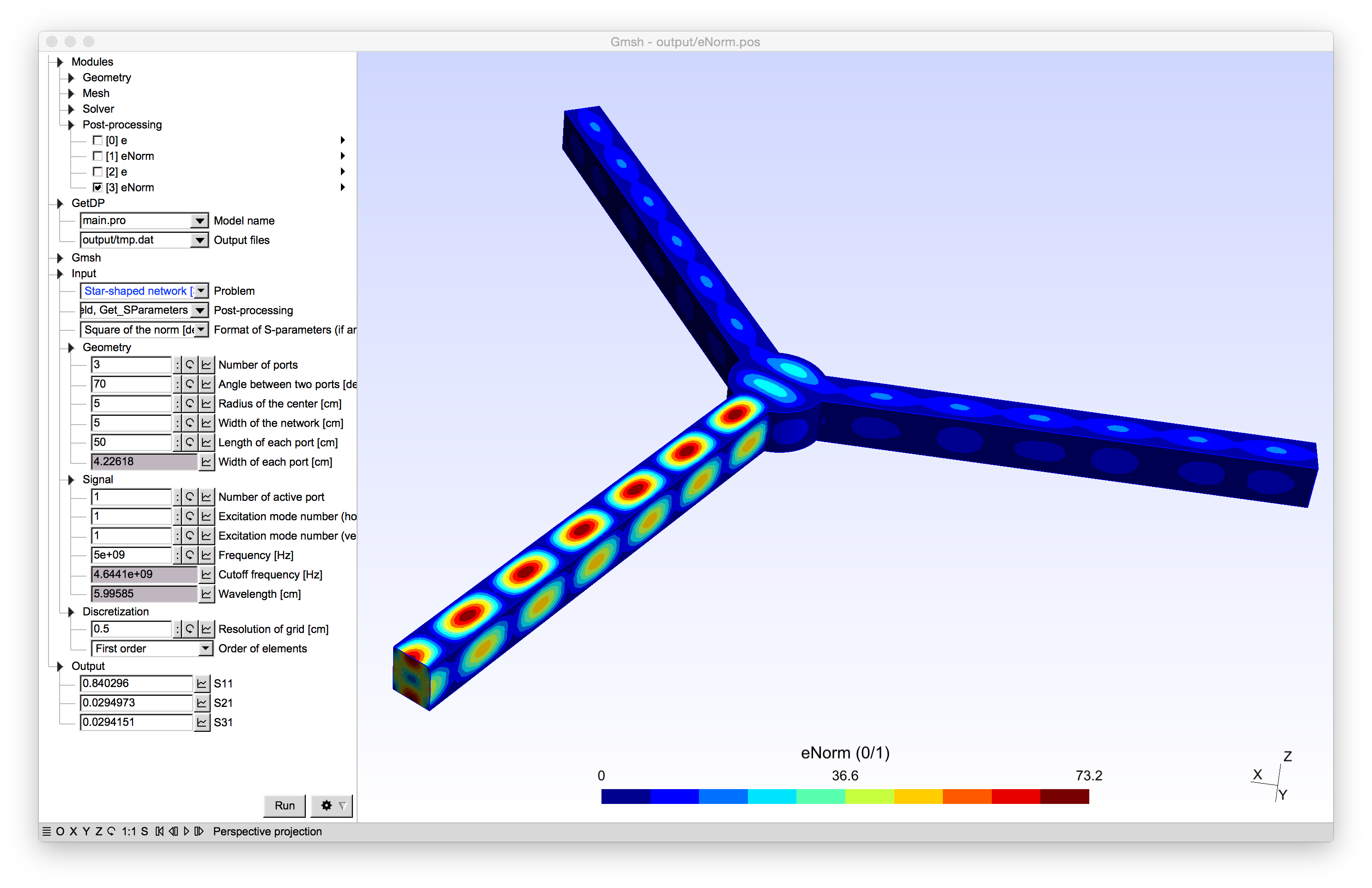
Some results
Here are some snapshots.
References
- ↑ 1.0 1.1 J. Jin, The Finite Element Method in Electromagnetics. Second edition. John Wiley & Sons, 2002
|
Model developed by A. Modave, B. Klein and C. Geuzaine
|