Tutorial/Eigenvalue problems

ERROR in secure-include.php: /onelab_files/academic_eigenvalues/README.txt does not look like a URL, and doesn't exist as a file.
Download model archive (academic_eigenvalues.zip) Browse individual model files

\(\renewcommand{\vec}[1]{\mathbf{#1}} \newcommand{\Grad}[1]{\mathbf{\text{grad}}\,{#1}} \newcommand{\Curl}[1]{\mathbf{\text{curl}}\,{#1}} \newcommand{\Div}[1]{\text{div}\,{#1}} \newcommand{\Real}[1]{\text{Re}({#1})} \newcommand{\Imag}[1]{\text{Im}({#1})} \newcommand{\pvec}[2]{{#1}\times{#2}} \newcommand{\psca}[2]{{#1}\cdot{#2}} \newcommand{\E}[1]{\,10^{#1}} \newcommand{\Ethree}{{\mathbb{E}^3}} \newcommand{\Etwo}{{\mathbb{E}^2}} \newcommand{\Units}[1]{[\mathrm{#1}]} \)

Introduction

This academic example introduces the numerical solution of eigenvalue problems. The Helmholtz equation (scalar and vector versions) is considered with homogeneous Dirichlet boundary conditions, for different basic geometries (i.e. linear, squared, circular and cuboid domain). These problems have a family of solutions. The eigenvalue solver used for this example provide the first eigenvalues and the associated eigenfunctions (i.e. the first possible solutions).

$\rightarrow$ To run the model, open main.pro with Gmsh.

Description of the model

Differential formulations

We consider differential problems based on the scalar and vector Helmholtz equations with homogeneous Dirichlet boundary conditions. Let the bounded domain $\Omega\subset\mathbb{R}^d$, whose boundary is denoted $\partial\Omega$.

• For the scalar-wave eigenvalue problem, we are looking for a scalar value $k$ and a scalar field $u(\mathbf{x})$ that are the solution of

\begin{equation} \begin{cases} \Delta u + k^2 u = 0 & \text{ in } \Omega,\\ u = 0 & \text{ on } \partial\Omega, \end{cases} \end{equation}

where $\Delta$ is the Laplace operator.

• For the vector-wave eigenvalue problem, we are looking for a scalar value $k$ and a vector field $\mathbf{u}(\mathbf{x})$ that are the solution of

\begin{equation} \begin{cases} \Delta \mathbf{u} + k^2 \mathbf{u} = 0 & \text{ in } \Omega, \\ \mathbf{n}\times\mathbf{u} = 0 & \text{ on } \partial\Omega, \end{cases} \end{equation}

where $\Delta$ is the vector version of the Laplace operator and $\mathbf{n}(\mathbf{x})$ is the outward unit normal to $\partial\Omega$.

The solution of these problems is not unique . There is a family of eigenvalues $k_i$ associated to eigenfunctions $u_i(\mathbf{x})$ or $\mathbf{u}_i(\mathbf{x})$ that solve these problems.

Finite element schemes

The eigenvalue problems are solved by using finite element schemes based on the following weak forms.

• For the scalar-wave problem, the weak form is

\begin{equation} \left\{ \begin{array}{l} \displaystyle{\text{Find } u \in H_0(\Omega,\Grad) \text{ such that}}\\ \displaystyle{\forall u'\in H_0(\Omega,\Grad),\qquad \int_{\Omega}\Grad u\cdot\Grad u'\;{\rm d}\Omega - \int_{\Omega}k^2 uu'\;{\rm d}\Omega =0,} \end{array}\right. \end{equation}

where $H_0(\Omega,\Grad) = \{v \in L_2(\Omega) \text{ such that } \Grad v \in \mathbf{L}_2(\Omega) \text{ and } v|_{\partial\Omega} = 0\}$.

• For the vector-wave problem, the weak form is (see e.g. , chapter 7)

\begin{equation} \left\{ \begin{array}{l} \displaystyle{\text{Find } \mathbf{u} \in H_0(\Omega,\Curl) \text{ such that}}\\ \displaystyle{\forall \mathbf{u}'\in H_0(\Omega,\Curl),\qquad \int_{\Omega} \Curl{\mathbf{u}}\cdot\Curl{\mathbf{u}'}\;{\rm d}\Omega - \int_{\Omega}k^2 \mathbf{u}\cdot\mathbf{u}'\;{\rm d}\Omega =0,} \end{array}\right. \end{equation}

where $H_0(\Omega,\Curl) = \{\mathbf{v} \in \mathbf{L}_2(\Omega) \text{ such that } \Curl{\mathbf{v}} \in \mathbf{L}_2(\Omega) \text{ and } \mathbf{n}\cdot\mathbf{v}|_{\partial\Omega} = 0\}$.

These formulations are coded in formulation.pro. The functional spaces are based on nodal elements for the scalar-wave problem (Form0) and edge elements for the vector-wave problem (Form1P in 1D and 2D, and Form1 in 3D). The homogeneous Dirichlet boundary condition are prescribed through constraints in the functional spaces.

Eigenvalue algebraic problem

The final discrete problem reads $$ [\vec{A}-k^2 \vec{I}] \vec{x} = \vec{0}, $$ where $\vec{x}$ contains all discrete unknowns of the problem. In GetDP, the eigenvalues and eigenvectors of this algebraic system are provided by numerical algorithms of SLEPc or ARPACK libraries.

Some results

Here are some snapshots of eigenfunctions for the scalar-wave eigenvalue problem with different domains.

• 

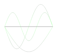
  First modes for the linear domain

• 

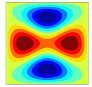
  One mode for the squared domain

• 

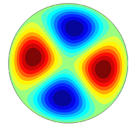
  One mode for the circular domain

• 

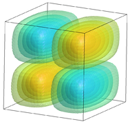
  One mode for the cuboidal domain

References

ERROR in secure-include.php: /onelab_files/academic_eigenvalues/COPYING.txt does not look like a URL, and doesn't exist as a file.

References

- ↑ L.C. Evans, Partial Differential Equations. Second edition. American Mathematical Society, 2010
- ↑ J. Jin, The Finite Element Method in Electromagnetics. Second edition. John Wiley & Sons, 2002